Overdamped Oscillator
Question
Solution
Short
Video
\(\LaTeX\)

No explanation / solution video to this exercise has yet been created.
Visit our YouTube-Channel to see solutions to other exercises.
Don't forget to subscribe to our channel, like the videos and leave comments!
Visit our YouTube-Channel to see solutions to other exercises.
Don't forget to subscribe to our channel, like the videos and leave comments!
Exercise:
A linearly damped oscillator can be described by the following system of differential s: fracddtleftmatrixy v_ymatrixright leftmatrix & -omega_^ & -deltamatrixright leftmatrixy v_ymatrixright abcliste abc Find the eigenvalues and eigenvectors. Show that the system corresponds to a stable node for deltaomega_ overdamped. abc Derive the solutions for the initial conditions yy_ v_y start from rest and y v_yv_ initial push. abcliste
Solution:
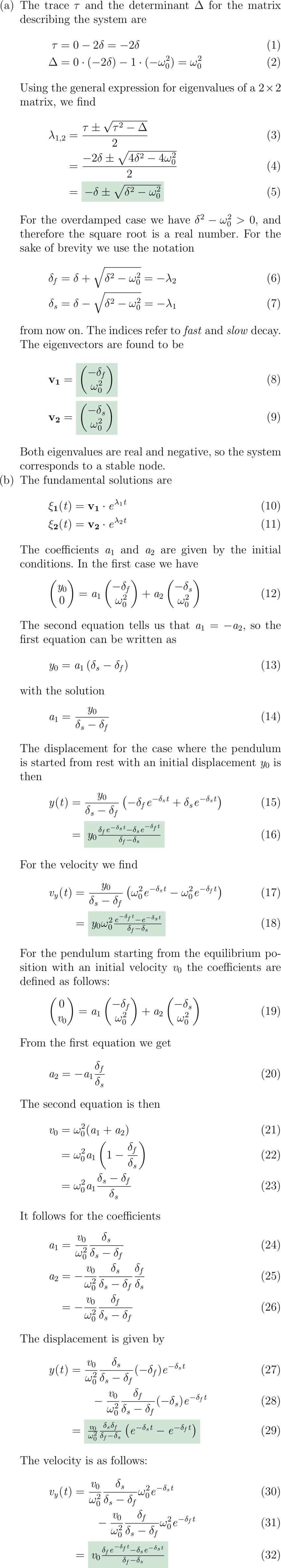
abcliste abc The trace tau and the determinant Delta for the matrix describing the system are tau -delta -delta Delta -delta--omega_^omega_^ Using the general expression for eigenvalues of a times matrix we find lambda_ fractaupmsqrttau^-Delta frac-deltapmsqrtdelta^-omega_^ result-deltapmsqrtdelta^-omega_^ For the overdamped case we have delta^-omega_^ and therefore the square root is a real number. For the sake of brevity we use the notation delta_f delta+sqrtdelta^-omega_^-lambda_ delta_s delta-sqrtdelta^-omega_^-lambda_ from now on. The indices refer to fast and slow decay. The eigenvectors are found to be bf v_ resultleftmatrix-delta_f omega_^ matrixright bf v_ resultleftmatrix-delta_s omega_^ matrixright Both eigenvalues are real and negative so the system corresponds to a stable node. abc The fundamental solutions are bf xi_t bf v_ e^lambda_ t bf xi_t bf v_ e^lambda_ t The coefficients a_ and a_ are given by the initial conditions. In the first case we have leftmatrixy_ matrixright a_ leftmatrix-delta_f omega_^ matrixright + a_ leftmatrix-delta_s omega_^ matrixright The second tells us that a_-a_ so the first can be written as y_ a_leftdelta_s -delta_fright with the solution a_ fracy_delta_s -delta_f The displacement for the case where the pulum is started from rest with an initial displacement y_ is then yt fracy_delta_s -delta_fleft-delta_f e^-delta_s t+delta_s e^-delta_s tright resulty_fracdelta_f e^-delta_s t-delta_s e^-delta_f tdelta_f-delta_s For the velocity we find v_yt fracy_delta_s-delta_fleftomega_^ e^-delta_s t-omega_^ e^-delta_f tright resulty_ omega_^frace^-delta_f t-e^-delta_s tdelta_f-delta_s For the pulum starting from the equilibrium position with an initial velocity v_ the coefficients are defined as follows: leftmatrix v_matrixright a_ leftmatrix-delta_f omega_^ matrixright + a_ leftmatrix-delta_s omega_^ matrixright From the first we get a_ -a_fracdelta_fdelta_s The second is then v_ omega_^ a_+a_ omega_^ a_ left-fracdelta_fdelta_sright omega_^ a_fracdelta_s-delta_fdelta_s It follows for the coefficients a_ fracv_omega_^fracdelta_sdelta_s-delta_f a_ -fracv_omega_^fracdelta_sdelta_s-delta_f fracdelta_fdelta_s -fracv_omega_^fracdelta_fdelta_s-delta_f The displacement is given by yt fracv_omega_^fracdelta_sdelta_s-delta_f-delta_f e^-delta_s t & quadquad -fracv_omega_^fracdelta_fdelta_s-delta_f-delta_s e^-delta_f t resultfracv_omega_^fracdelta_sdelta_fdelta_f-delta_slefte^-delta_s t-e^-delta_f tright The velocity is as follows: v_yt fracv_omega_^fracdelta_sdelta_s-delta_f omega_^ e^-delta_s t & quadquad -fracv_omega_^fracdelta_fdelta_s-delta_f omega_^ e^-delta_f t resultv_ fracdelta_f e^-delta_f t-delta_s e^-delta_s tdelta_f-delta_s abcliste
A linearly damped oscillator can be described by the following system of differential s: fracddtleftmatrixy v_ymatrixright leftmatrix & -omega_^ & -deltamatrixright leftmatrixy v_ymatrixright abcliste abc Find the eigenvalues and eigenvectors. Show that the system corresponds to a stable node for deltaomega_ overdamped. abc Derive the solutions for the initial conditions yy_ v_y start from rest and y v_yv_ initial push. abcliste
Solution:
abcliste abc The trace tau and the determinant Delta for the matrix describing the system are tau -delta -delta Delta -delta--omega_^omega_^ Using the general expression for eigenvalues of a times matrix we find lambda_ fractaupmsqrttau^-Delta frac-deltapmsqrtdelta^-omega_^ result-deltapmsqrtdelta^-omega_^ For the overdamped case we have delta^-omega_^ and therefore the square root is a real number. For the sake of brevity we use the notation delta_f delta+sqrtdelta^-omega_^-lambda_ delta_s delta-sqrtdelta^-omega_^-lambda_ from now on. The indices refer to fast and slow decay. The eigenvectors are found to be bf v_ resultleftmatrix-delta_f omega_^ matrixright bf v_ resultleftmatrix-delta_s omega_^ matrixright Both eigenvalues are real and negative so the system corresponds to a stable node. abc The fundamental solutions are bf xi_t bf v_ e^lambda_ t bf xi_t bf v_ e^lambda_ t The coefficients a_ and a_ are given by the initial conditions. In the first case we have leftmatrixy_ matrixright a_ leftmatrix-delta_f omega_^ matrixright + a_ leftmatrix-delta_s omega_^ matrixright The second tells us that a_-a_ so the first can be written as y_ a_leftdelta_s -delta_fright with the solution a_ fracy_delta_s -delta_f The displacement for the case where the pulum is started from rest with an initial displacement y_ is then yt fracy_delta_s -delta_fleft-delta_f e^-delta_s t+delta_s e^-delta_s tright resulty_fracdelta_f e^-delta_s t-delta_s e^-delta_f tdelta_f-delta_s For the velocity we find v_yt fracy_delta_s-delta_fleftomega_^ e^-delta_s t-omega_^ e^-delta_f tright resulty_ omega_^frace^-delta_f t-e^-delta_s tdelta_f-delta_s For the pulum starting from the equilibrium position with an initial velocity v_ the coefficients are defined as follows: leftmatrix v_matrixright a_ leftmatrix-delta_f omega_^ matrixright + a_ leftmatrix-delta_s omega_^ matrixright From the first we get a_ -a_fracdelta_fdelta_s The second is then v_ omega_^ a_+a_ omega_^ a_ left-fracdelta_fdelta_sright omega_^ a_fracdelta_s-delta_fdelta_s It follows for the coefficients a_ fracv_omega_^fracdelta_sdelta_s-delta_f a_ -fracv_omega_^fracdelta_sdelta_s-delta_f fracdelta_fdelta_s -fracv_omega_^fracdelta_fdelta_s-delta_f The displacement is given by yt fracv_omega_^fracdelta_sdelta_s-delta_f-delta_f e^-delta_s t & quadquad -fracv_omega_^fracdelta_fdelta_s-delta_f-delta_s e^-delta_f t resultfracv_omega_^fracdelta_sdelta_fdelta_f-delta_slefte^-delta_s t-e^-delta_f tright The velocity is as follows: v_yt fracv_omega_^fracdelta_sdelta_s-delta_f omega_^ e^-delta_s t & quadquad -fracv_omega_^fracdelta_fdelta_s-delta_f omega_^ e^-delta_f t resultv_ fracdelta_f e^-delta_f t-delta_s e^-delta_s tdelta_f-delta_s abcliste